Object Detection
Vehicular and Non-Vehicular Object Detection
Motivation: This project deals with detecting different
Motivation: This project deals with detecting different
Our main motive to do this project is to compare different algorithms which works better for our required needs. To identify all the objects in an image provided and divide them into vehicular and non vehicular so that we can know the density of the vehicles in an busy day or in any daily situations we face. We aim to further divide vehicle into categories on the basis of their size .
1)You can know what type of vehicles are coming on to roads.
2)You can control traffic using the results we got from this method.
Overview:
Our main idea in this project is
to detect all the appropriate objects in a selected image and further classify
them. We are using various techniques like deep learning and machine learning
to detect and classify the objects.
Working:
Here we have used many methods for object
detection part of our project. The following flow chart (figure1) gives a brief idea about our project.

YOLO
v3:
Here we are using “YOLOv3”
because it is far more better than other versions of YOLO. YOLOv3 has come with
better feature extraction, as well as a better object detection with feature
mapping and upsampling (As you can see in figure2) . It also uses Darknet-53 framework
with more shortcut connections.

Outline of YOLOv3:
Algorithm
and architecture:
Yolov3 uses an algorithm that
uses convolutional neural networks for object detection. It is not the most
accurate object detection algorithm, but when we talk about real-time
situations, it will be a very good choice for detection. This detection algorithm
doesn’t only predict class labels but also detects locations of objects within
a image and classifies the image into a category. The architecture is very
simple in this case. This network divides the image into regions and predicts
the bounding boxes for them.
Bounding box
prediction:
Here the parameters like x, y, w,
h are predicted. Also objectness score is predicted using logistic regression.
It is considered as 1 if the bounding box prior overlaps a ground truth object
by more than any other bounding box prior. Only 1 bounding box prior is
assigned for each ground truth object.
Convolution neural network:
Yolov3 uses only convolutional layers, making it fully convolutional network. It includes darknet-53, as it name says it contains 53 convolutional layers each followed by normalization layer. In this architecture no form of pooling is used and a convolutional layer with a stride 2 is used to downsample the feature maps. This is useful in preventing loss of low-level features.
In this we are not using any kind
of softmax. Instead we use independent logistic classifiers and binary cross
and entropy loss are used. Because there may be overlapping for multilabel
classification if YOLOv3 is moved to any other complex domain such as Open
images dataset.
As you can see in the figure3.

Prediction
across scales:
Here in YOLOv3 we have used coco
dataset. Many convolution layers are being added to the feature extractor
darknet-53. The last three layers predicts the bounding box, objectness and
class predictions. On coco dataset the output is represented by
N*N*[3*(4+1+80)]
Here 3
represents number of boxes at each scale
4
represents bounding box offsets
1
represents the objectness
80 is
nothing but class predictions
YOLOv3 can identify more than 80 different objects in a
single image.
Darknet-53:
Here in YOLOv3 we use darknet-53
framework. In YOLOv2 we have used darknet-19 framework but
when compared to this darknet-53 is much more better. Because it is much
deeper network with 53 convolution layers.

Figure4
The shortcut connections are also shown in figure 4(it is an
example of darknet layers)
Why YOLOv3 is better than other
versions?
YOLOv3 is more preferable for object detection
when compared to YOLOv1 and YOLOv2. This is because of its more features like
upsampling and concatenation.( Concatenation means the ability to link up the
things together which made YOLOv3 more special) And also in other versions of
YOLO they couldn’t find the small objects if they appear as a cluster. Moreover
the localization of objects in input image is being very difficult in those
versions. These issues have been solved in YOLOv3. The background error has
also reduced in this version.
YOLOv3 has also improved in the
stability of neural network by decreasing the shift in unit value in the hidden
layers. It has also improved the mean average precision. This version has an
ability to train with random images with different dimensions. The problem of
overfitting has also been reduced in this version.
Faster
RCNN :
There are some lower version of this method like RCNN ,Fast RCNN but due to some advanced methods
in the process Faster RCNN works better than remaining two methods.
Let’s understand the process through a flow chart:

·
Convolution layer :
In this layers we train
filters to extract the appropriate features the image. You feed whole image to
this layer at once to extract features . Convolution networks are generally
composed of Convolution layers, pooling layers and a last component which is
the fully connected or another extended thing that will be used for an appropriate
task like classification or detection.

In the (figure5 figure6
figure7) you can see how convolution
works between the input image and filters. Similar to this there are so many
filters in convolution layer for different feature extraction from the given
input image.
REGION PROPOSAL NETWORKS (
RPN ):
A Region Proposal Network (RPN) takes an image
(of any size) as input and outputs a set of rectangular object proposals, each
with an objectness score. It is the think that differs Faster RCNN from Fast
RCNN , In fast RCNN we use selective search algorithm to divide image into
regions bbut here we use a separate network called RPN
map output by the last shared convolutional layer. This
small network takes as input an n × n spatial window of the input convolutional
feature map. Each sliding window is mapped to a lower-dimensional feature (
512-d for VGG archietecture)
Each of the sliding window [10] has an anchor centered with
different sizes and aspect ratios, so we have a total of W*H*k anchors where W
and H are width and height of the anchors respectively and k is the number of
anchors. These anchors provide us a cost efficient way to get the region
proposals by using a pyramid approach.
ROI POOLING AND SOFTMAX LAYER
:
ROI pooling layer we reshape
them into a fixed size so that it can be fed into a fully connected layer. From
the ROI feature vector, we use a softmax layer to predict the class of the
proposed region and also the offset values for the bounding box.

Figure7 shows how faster rcnn work step by step
After getting region
proposals you give it to ROI pooling and then softmax from which you’ll
identify your bounding boxes acroos images.
From this you’ll get the
output
Difference between RCNN ,
FAST RCNN , FASTER RCNN :
You have seen faster RCNN
flow chart above , there we fed whole image to convolution layer and then
divided into regions . RCNN differs from fast RCNN and faster RCNN in this
matter . In RCNN , first we divide the image into regions using SELECTIVE
SEARCH and then give regions to CNN layer .
Difference between Fast RCNN
and FASTER RCNN is to divide convolution feature map into regions we use SELECTIVE
ALGORITHM in FAST RCNN and RPN in
FASTER RCNN.
Faster RCNN takes 0.2 seconds
to detect object whereas Fast RCNN takes 2.3 secs and RCNN takes 23 secs . This
huge difference comes in between faster RCNN and RCNN because we feed a whole
image to CNN layer whole at once but In RCNN you feed regions to CNN layer
which consumes a lot of time.

Figure8 explains the architecture of Faster RCNN
Bbox regressor at the output :
Predict localization boxes in recent object detection
approaches. Typically, bounding-box regressors are trained to regress from
either region proposals or fixed anchor boxes to nearby bounding boxes of a
pre-defined target object classes.
SINGLE
SHOT MULTIBOX DETECTION (SSD ) :
Here it takes one songle shot to detect multiple object
within image unlike RCNN which dives image into multiple regions and work on
them individually.
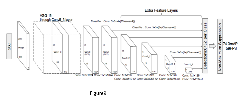
Figure9 is the architecture of SSD.
It uses VGG16 as it’s base network instead of fully
connected layer because of VGG16 ability to perform high quality image
classification
Instead of the original VGG
fully connected layers, a set of auxilary convolutional layers
(from conv6 onwards) were added, thus enabling to extract features
at multiple scales and progressively decrease the size of the input to each such
subsequent layer.
Multy box :
It is a bounding box
regression technique of SSD.
MultiBox’s loss function also combined two critical
components that made their way into SSD:
Confidence
Loss: this measures
how confident the network is of the objectness of the computed bounding box.
Categorical cross-entropy is
used to compute this loss.
Location
Loss: this
measures how far away the
network’s predicted bounding boxes are from the
ground truth ones from the
training set.
multibox_loss = confidence_loss + alpha * location_loss
The alpha term helps
us in balancing the contribution of the location loss.It depends on the how
much you want to cover here.
Multibox Prior and IoU:
The logic revolving around
the bounding box generation is actually more complex .
Priors, which are
pre-computed, fixed size bounding boxes that closely match the distribution of
the original ground truth boxes. In fact those priors are selected in such a way that their
Intersection over Union ratio ( IoU
) is greater than 0.5 .
MultiBox
starts with the priors as predictions and attempt to regress closer to the
ground truth bounding boxes.

From figure10 you can understand multibox detection ,prior
and IoU.
CENTERNET :
It is an extension of corner net . Here center net also uses
region proposals .It uses the center part of the region proposal to detect the object. Here center
pooling uses center keypoint along with corner points to obtain more recognisable patterns of
object.

Here’s(figure11) the archietecture of centernet. It uses
triplet points to detect the object that is (x,y) co-ordinates of a corner and
center of the object bounding box . We use hourglass archeitecture as backbone
layer.
The work states that if a predicted bounding box has a high
IoU with the ground-truth box, then the probability that the center keypoint in
its central region is predicted as the same class is high, and vice versa.
During inference, given the corner points as the proposals, the network
verifies whether the corner proposal is indeed an object by checking if there’s
a center key point of the same class falling within its central region. The
additional use of object centeredness keeps the network as one stage detector
but inherits the functionality of RoI polling like it’s used in two-stage
detectors.
Center Pooling :
A new pooling method is
proposed to capture richer and more recognizable visual patterns. This method
is required since the center point of the object does not necessarily convey
very recognizable visual patterns.Given the feature map from the backbone
layer, we determine if a pixel in the feature map is a center keypoint. The pixel in the feature map
itself does not contain enough centeredness information of the object.
Therefore, the maximum value of both horizontal and vertical directions are
found and added together.
Cascade Corner Pooling :
In the CornerNet paper, corner pooling is
proposed to capture local appearance features in the corner points of the
objects. Unlike center pooling that takes maximum values in both horizontal and
vertical directions, corner pooling only takes the maximum values in boundary
directions but
this makes corner edges sensitive as we are only consdidering maximum
values.this problem is solved by using cascade corner pooling. it first
looks along a boundary to find a boundary maximum value, then looks inside
along the location of the boundary maximum value to find an internal maximum
value, and finally, adds two maximum values together which reduces the
sensitiveness of the edges detection.

Conclusion:
In this project we understood different algorithms and tools to detect the object and classify them and compare which is faster and more accurate among all the tools. We also develop an app and include which of the following algorithm is better and faster one into that app so it can be easy for the user to detect the image at that particular instance of time.
References :
centernet
– towardsdatscience (https://towardsdatascience.com/centernet-keypoint-triplets-for-object-detection-review-a314a8e4d4b0)
faster
RCNN – towardsdatscience (https://towardsdatascience.com/faster-rcnn-object-detection-f865e5ed7fc4)
faster RCNN reasearch paper (https://papers.nips.cc/paper/5638-faster-r-cnn-towards-real-time-object-detection-with-region-proposal-networks.pdf)
yolov3 - towardsdatscience (https://towardsdatascience.com/review-yolov3-you-only-look-once-object-detection-eab75d7a1ba6)
yolov3 -
towardsdatascience by (https://towardsdatascience.com/@ManishChablani)


Comments
Post a Comment